The Great FFT
Table of Contents
Every time you make a phone call, compress an image, or use noise-canceling headphones, you're benefiting from one algorithm: the Fast Fourier Transform. If you're in software, you've probably wondered: What are the coolest algorithms ever discovered? As a fun exploration, I decided to understand SIAM's top 10 algorithms of the 20th century.
The Fast Fourier Transform (FFT) algorithm is revolutionary. Its applications touch nearly every area of engineering. The Cooley-Tukey paper rediscovered (it was originally found in Gauss's notes for astronomical calculations!) and popularized FFT. It remains one of the most widely cited papers in science and engineering.
FFT is something I've used extensively but never fully understood. I always thought of it as something that makes the Fourier transform faster for viewing time-domain signals in frequency domain. While that's one application, the key insight is much broader: FFT is fundamentally about making polynomial operations blazingly fast.
Polynomials
A polynomial is an expression of the form:
\[ A(x) = a_0 + a_1x + a_2x^2 + a_3x^3 + \ldots + a_{n-1}x^{n-1} \]
where \(a_i\) are coefficients (typically real numbers) and \(x\) is a variable. This polynomial \(A(x)\) has degree \(n-1\) (one less than the number of terms).
Representing Polynomials
How can we represent polynomials in a computer? There are two fundamental approaches:
Coefficient Representation
\[ (a_0, a_1, a_2, \ldots, a_{n-1}) \]
Simple—it's just a vector of numbers! This representation handles any one-dimensional data naturally. We can write a function \(A(x)\) to evaluate the polynomial, or simply work with the coefficients as a vector.
Point-Value Representation
\[(x_0, y_0), (x_1, y_1), (x_2, y_2), \ldots, (x_{n-1}, y_{n-1})\]
Since a polynomial \(A(x)\) is a function mapping \(x\) to \(y\), we can represent it using input-output pairs. But do we need to define \(A(x)\) at all possible values? No! There's a fundamental property:
Given \(n\) pairs \((x_0,y_0), (x_1,y_1), \ldots, (x_{n-1},y_{n-1})\) where all \(x_i\)'s are distinct, there exists a unique polynomial \(p(x)\) of degree at most \(n-1\) such that \(p(x_i) = y_i\) for all \(i\).
Intuitively, this makes sense. A line requires 2 points, a parabola needs 3 points, and so on. A polynomial of degree \(n-1\) is uniquely determined by \(n\) point-value pairs. You can find a proof here.
Operations on Polynomials
What can we do with polynomials?
Evaluation
Given polynomial \(p\) and number \(x\), compute \(p(x)\).
Addition
Given polynomials \(p(x)\) and \(q(x)\), find polynomial \(r = p + q\) such that \(r(x) = p(x) + q(x)\) for all \(x\). If both have degree \(n-1\), the sum also has degree at most \(n-1\).
Multiplication
Given polynomials \(p(x)\) and \(q(x)\), find polynomial \(r = p \cdot q\) such that \(r(x) = p(x) \cdot q(x)\) for all \(x\). If both have degree \(n-1\), the product has degree \(2n-2\).
Complexity Analysis
Let's analyze the time complexity for each representation:
Coefficient Representation
Evaluation: Simple loop achieves \(O(n)\) operations (can be optimized further with Horner's method).
Addition: Element-wise addition in \(O(n)\) operations.
Multiplication: This is the bottleneck—requires \(O(n^2)\) operations using the standard algorithm. While advanced techniques exist, they have large constants.
Point-Value Representation
Addition: Given polynomials \((x_i, y_i)\) and \((x_i, z_i)\), simply compute \((x_i, y_i + z_i)\). This takes \(O(n)\) operations.
Note: Both polynomials must be evaluated at the same points, otherwise we need Lagrange interpolation.
Multiplication: Given polynomials \((x_i, y_i)\) and \((x_i, z_i)\), compute \((x_i, y_i \cdot z_i)\). This takes \(O(n)\) operations.
Note: Multiplying two degree-\((n-1)\) polynomials yields a degree-\((2n-2)\) polynomial, so we need more sample points. We handle this by evaluating both input polynomials at \(2n-1\) points before multiplication.
Evaluation: To evaluate at a new point requires interpolation, which takes \(O(n^2)\) operations.
Summary
| Representation | Multiplication | Evaluation | Addition |
|---|---|---|---|
| Coefficient | \(O(n^2)\) | \(O(n)\) | \(O(n)\) |
| Point-Value | \(O(n)\) | \(O(n^2)\) | \(O(n)\) |
The question becomes: Can we convert between representations efficiently to get the best of both worlds? This is exactly where FFT shines.
Converting Between Representations
For polynomial \(A(x) = a_0 + a_1x + \ldots + a_{n-1}x^{n-1}\), converting from coefficient to point-value representation at \(n\) distinct points \((x_0, x_1, \ldots, x_{n-1})\) can be expressed as:
\begin{bmatrix} y_0 \\ y_1 \\ \vdots \\ y_{n-1} \end{bmatrix} = \begin{bmatrix} 1 & x_0 & x_0^2 & \cdots & x_0^{n-1} \\ 1 & x_1 & x_1^2 & \cdots & x_1^{n-1} \\ \vdots & \vdots & \vdots & \ddots & \vdots \\ 1 & x_{n-1} & x_{n-1}^2 & \cdots & x_{n-1}^{n-1} \end{bmatrix} \begin{bmatrix} a_0 \\ a_1 \\ \vdots \\ a_{n-1} \end{bmatrix}This is the Vandermonde matrix \(V\). The conversion is \(\vec{y} = V\vec{a}\) and requires \(O(n^2)\) operations.
To convert back from point-value to coefficient representation, we compute \(\vec{a} = V^{-1}\vec{y}\), which also takes \(O(n^2)\) operations.
Fact: \(V\) is invertible when all \(x_i\)'s are distinct.
The Key Insight
Here's the crucial observation: we get to choose the sample points \(x_i\) in matrix \(V\)! If we pick these values with the right structure, maybe this conversion can be much faster. We're trading generality for speed, but we don't care—we still get efficient conversion between representations.
FFT exploits this freedom of choice.
Divide and Conquer Strategy
Our Goal
Let's be crystal clear about what we want:
- We have polynomial \(A(x)\) in coefficient form \(\langle a_0, a_1, \ldots, a_{n-1} \rangle\)
- We have an input set \(X\) of \(n\) points
- We need to compute \(\langle y_0, y_1, \ldots, y_{n-1} \rangle\) where \(y_i = A(x_i)\) for all \(x_i \in X\)
- The key insight: we're free to choose the input set \(X\)
The essence of divide and conquer is:
- Divide: Split problem into smaller subproblems
- Conquer: Recursively solve subproblems
- Combine: Merge solutions into solution for original problem
Divide and Conquer for Polynomials
Consider polynomial \(A(x) = a_0 + a_1x + a_2x^2 + \ldots + a_7x^7\).
Divide: Express \(A(x)\) as sum of odd and even powers: \[ A_{\text{even}}(x) = a_0 + a_2x + a_4x^2 + a_6x^3 \] \[ A_{\text{odd}}(x) = a_1 + a_3x + a_5x^2 + a_7x^3 \]
Conquer: Recursively compute \(A_{\text{even}}(z)\) and \(A_{\text{odd}}(z)\) for all \(z \in \{x^2 | x \in X\}\)
Combine: Use the identity: \[ A(x) = A_{\text{even}}(x^2) + x \cdot A_{\text{odd}}(x^2) \]
This requires only one multiplication and one addition—\(O(1)\) operations!
Base case: Stop when polynomial has degree 0 (one coefficient).
Note: We evaluate both \(A_{\text{even}}\) and \(A_{\text{odd}}\) at \(x^2\). This is crucial for the math to work out.
Making Subproblems Smaller
For divide and conquer to be effective, subproblems must be smaller than the original. We need the set \(Z = \{x^2 | x \in X\}\) to have fewer elements than \(X\).
Can we find a set of \(n\) points such that squaring each element produces a smaller set?
For \(n = 2\): If \(X = \{a, -a\}\), then \(Z = \{a^2\}\) has size 1. This works!
For \(n = 4\): We need 4 points that become 2 points when squared. This is where complex numbers become essential.
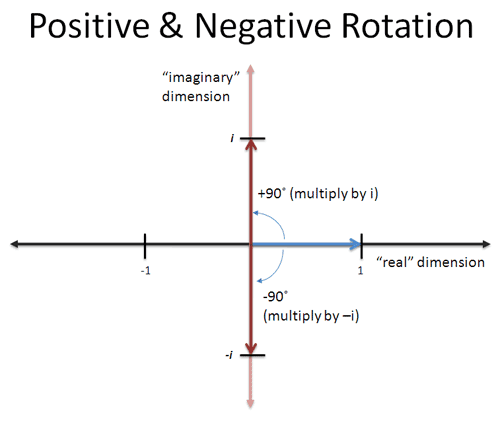
Enter Complex Numbers
Think of complex numbers as rotations in the plane. The key insight from Kalid's excellent explanation is that complex numbers represent rotations around the origin.
Let's build our collapsing sets:
- \(S_1 = \{1\}\) (size 1)
- \(S_2 = \{1, -1\}\) (size 2, squares to \(S_1\))
- \(S_4 = \{1, -1, i, -i\}\) (size 4, squares to \(S_2\))
- \(S_8 = \{1, -1, i, -i, \frac{1+i}{\sqrt{2}}, \frac{-1-i}{\sqrt{2}}, \frac{i-1}{\sqrt{2}}, \frac{-i+1}{\sqrt{2}}\}\) (size 8, squares to \(S_4\))
We can continue this pattern indefinitely! For any power of 2, we can find a set that "collapses" by half when squared.
These special sets are called the nth roots of unity —they're the \(n\) complex numbers that, when raised to the \(nth\) power, equal 1.
Runtime Analysis
Let's analyze our divide-and-conquer algorithm:
- Take polynomial \(A(x)\) to be evaluated on set \(X\) with \(|X| = n\)
- Reduce to two subproblems: \(A_{\text{even}}\) and \(A_{\text{odd}}\), both evaluated on set \(Y = \{x^2 | x \in X\}\) with \(|Y| = n/2\)
- Combine solutions in \(O(n)\) time
The recurrence relation is: \[T(n) = 2T(n/2) + O(n)\]
Solving this recurrence, we get \(T(n) = O(n \log n)\).
Remarkable! We can now perform polynomial addition, evaluation, and multiplication in \(O(n \log n)\) time by:
- Converting to point-value representation using FFT (\(O(n \log n)\))
- Performing the operation (\(O(n)\))
- Converting back to coefficient representation using inverse FFT (\(O(n \log n)\))
This elegant divide-and-conquer algorithm is the essence of the Fast Fourier Transform!
Looking Forward
This explanation focused on the core algorithmic insight behind FFT. In future posts, we'll explore:
- Implementation details and the role of \(e^{i\theta}\)
- How this connects to traditional Fourier analysis
- Practical applications in signal processing, image compression, and beyond
The beauty of FFT lies not just in its efficiency, but in how it reveals deep connections between seemingly different mathematical concepts: polynomials, complex numbers, and harmonic analysis.