If you are in the field of software, you've probably wondered at some point: What are the coolest algorithms ever discovered?. As a fun task, I decided to try and understand SIAM's top 10 algorithms of the 20th century.
The Fast Fourier Transform (FFT) algorithm is revolutionary. The applications of FFT touches nearly every area of engineering in some way. The Cooley-Tukey paper rediscovered (It was found in Gauss's notes for calculations in astronomy! 🤷) and popularized FFT. It is one of the most widely cited papers in science and engineering!
FFT is something I've used a lot, but didn't quite understand fully. I always thought of it as something that makes the Fourier transform faster, in order to view time domain signals in their frequency domain. In reality, that is just one application of FFT. For me, the key view point was: FFT is all about making basic polynomial operations fast!.
Polynomials
A Polynomial is an expression of the form
$$ A(x) = a_0 + a_1x + a_2x^2 + a_3x^3 + ... a_{n-1}ax^{n-1} $$
where $a_i$ are Real numbered coefficients(typically) and $x$ is some variable. $A(x)$ is defined to have a degree of n-1 (Yup, one less than the number of terms!)
Representation of Polynomials
How can polynomials be represented in a computer?
Coefficient Representation $$ (a_0, a_1, a_2 ... a_{n-1}) $$ Simple enough, its a vector or list of numbers! This representation is often very useful, as it can represent any kind of one-dimensional data. Sure, if we care about $x$, we can write a function $A(x)$ to take some variable $x$ and do something with $x$ and these coefficents. If not, we just keep it as a vector.
Point-Value Representation $$(x_0, y_0), (x_1, y_1), (x_2, y_2), ... (x_{n-1}, y_{n-1})$$ Since a polynomial $A(x)$ can be thought of as a function from $x$ to $y$, another way to represent a polynomial would be by pairs of (input, output) values. Wow! Are you saying we need to define $A(x)$ at all possible values of $x$? Nope, it turns out there is a fundamental property of polynomials that states that:
Given $n$ pairs $(x_0,y_0)(x_{n-1},y_{n-1}),...$ all the $x_i$'s distinct, there is a unique polynomialn p(x) of degree (at most) n such that $p(x_i) = y_i$ for $0 \le i \le (n-1)$./
In other words, a polynomial of degree $(n-1)$ is uniquely specified by giving $n$ point-value pairs. Intuitively, that makes sense. How many points do we need to represent a line (which can be represented as a polynomial of the form $y = ax + b$)? 2 points! What continuous curve can we draw through 3 points? parabola! A proof can be found here.
What can we do with a Polynomial?
Evaluation
Given a polynomial $p$ and a number x, compute p(x).
Addition
Given two polynomials $p(x)$ and $q(x)$, find a polynomial $r = p + q$, such that $r(x) = p(x) + q(x)$ for all $x$. If $p$ and $q$ both have degree $n$, then the sum also has degree $n$.
Multiplication
Given two polynomials $p(x)$ and $q(x)$, find a polynomial $r = pq$, such that $r(x) = p(x).q(x)$ for all $x$. If $p$ and $q$ both have degree $n$, then the product has degree $2n$.
Complexity of these operations
Assuming the polynomials are represented using the coefficient representation:
Evaluation: A simple for-loop can achieve this in O(n) arithmetic operations. (We can cut down the multiplications further using horner's scheme.
Addition: A simple for-loop can achieve this in O(n) arithmetic operations.
Multiplication: Ha! this is more complicated and takes O($n^2$) arithmetic operations. (Sure, we can reduce the asymptotic runtime by using some fancy tricks, but the constants are still pretty large.)
What if we change the representation to point-value?
Addition: Simple! Given 2 polynomials, $(x_1, y_1), (x_2, y_2), . . . (x_{n-1}, y_{n-1})$ and $(x_1, z_1), (x_2, z_2), . . . (x_{n-1}, z_{n-1})$ we simply add the output values and get $(x_i, y_i + z_i)$. Thus, it requires $O(n)$ arithmetic operations.
Note: Both polynomials need to be defined for the same n points, else we'll have to do a little more work using Lagrange interpolation.
Multiplication: Simple! Given, 2 polynomials $(x_1, y_1), (x_2, y_2), . . . (x_{n-1}, y_{n-1})$ and $(x_1, z_1), (x_2, z_2), . . . (x_{n-1}, z_{n-1})$ we simply multiply the output values and get $(x_i, y_i * z_i)$. Thus, it requires $O(n)$ arithmetic operations.
Note: When we multiply 2 polynomials, we are going to get a polynomial of higher degree, so we'll need more points to represent it. For example, multiplying 2 $(n-1)$ degree polynomials will result in a polynomial of degree (2n - 1). This can be handled by taking more samples of the 2 input polynomials before multiplication
Summary
So this is where we are:
| Representation | Multiply | Evaluate | Sum |
|---|---|---|---|
| Coefficient | $O(n^2)$ | $O(n)$ | $O(n)$ |
| Point-Value | $O(n)$ | $O(n^2)$ | $O(n)$ |
Can we somehow convert between the representations efficiently so that we get the best of both? This is where the FFT comes in!
Converting between representations
For a polynomial $A(x) = a_0 + a_1x + ... a_{n-1}x^{n-1}$ of degree $(n-1)$, the conversion from coefficient representation to point-value representation at n distinct points $(x_0, x_1, ... x_n)$ can be done as follows:
$$
\begin{bmatrix} y_0 \\ y_1 \\ .\\ .\\ .\\ y_{n-1} \\ \end{bmatrix} = \begin{bmatrix} 1 & x_0 & x_0^2 & ... & x_0^{n-1} \\ 1 & x_1 & x_1^2 & ... & x_1^{n-1} \\ .\\ .\\ .\\ 1 & x_{n-1} & x_{n-1}^2 & ... & x_{n-1}^{n-1} \\ \end{bmatrix} \begin{bmatrix} a_0 \\ a_1 \\ .\\ .\\ .\\ a_{n-1} \\ \end{bmatrix}$$
where $\vec{a}$ is a vector of coefficients and $\vec{y}$ is a vector of output values. This is known as the Vandermonde matrix. It's a nice way of vectorizing the conversion and make the runtime $O(n^2) operations$. Thus, if we need the $y_i$ values for point-value representation, we simply do $$\vec{y} = V\vec{a}$$
To convert from point-value to coefficient representation, we take the inverse of $V^{-1}$.
$$V^{-1}\vec{y} = \vec{a}$$
Fact: $V$ is inverttible if $x_i$'s are distinct.
Anyways, the point is, the forward and reverse conversion takes $O(n^2)$ operations.
Can we do better?
If you look at the above matrix-vector product hard enough, you'll notice that we get to pick the x values in $V$. i.e The sample positions! If we pick these sample values with the 'right structure', maybe this conversion can be faster. Sure, it is not very generic, but we don't care! We still get to convert between point-value $\leftrightarrow$ coefficient representation of the given polynomial.
FFT exploits this freedom
Divide and Conquer!
What is our goal?
Before we lose the forest for the trees, this is what we want:
- We have a polynomial $A(x)$ in its coefficient form $<a_0, a_1, . . . a_{n-1}>$ and a input set $X$.
- We need to compute $<y_0, y_1, . . . y_{n-1}$ from $A(x) \forall x \in X$.
- The reason we want to do this, is so that we can quickly switch from coefficient to polynomial representation. (And vice-versa, but we'll leave that for now)
- The key insight from the previous section was that we are free to choose the input set $X$.
Ok, now back to divide and conquer.
The essence of any divide and conquer algorithm strategy is as follows:
- Divide problem into smaller subproblems.
- Recursively solve (conquer) the subproblems.
- Combine solutions to the subproblem into one for the original problem.
The above link gives some basic examples in this paradigm.
Divide and Conquer idea for Polynomials
Consider the polynomial $A(x) = a_0 + a_1x + a_2x^2 + . . . a_{7}x^{7}$.
- Divide
Express $A(x)$ as a sum of its odd and even powers.
$$ A_{even}(x) = a_0 + a_2x + a_4x^2 + a_6x^3 $$ $$ A_{odd}(x) = a_1 + a_3x + a_5x^2 + a_7x^3 $$
- Conquer
Recursively compute $A_{even}(z)$ and $A_{odd}(z)$ $\forall z \in \{ x^2 | x \in X \}$
- Combine
Combine them with $O(1)$ arithmetic operations (Specifically, 1 multiplication and 1 addition) to get $A(x)$!
$ A(x) = A_{even}(x^2) + xA_{odd}(x^2) $
Basecase: We stop recursing, when our polynomial just has 1 coefficient
Note that we evaluate both $A_{even}$ and $A_{odd}$ at $x^2$ for the numbers to work out. That's key.
Do we have smaller a subproblems?
i.e, is $A_{even}(z)$ and $A_{odd}(z)$ $\forall z \in \{ x^2 | x \in X \}$ smaller than $A(x) \forall x \in X$?
If we look at the the set of input values on which $A_{even}$ and $A_{odd}$ are evaluated, we still need them to be defined for all values of $x^2$.
For the divide and conquer technique to work, we need the subproblems to be of a smaller size.
Can we find a set of $n$ points such that the set formed by squaring each value, is a smaller set?
If my set $X = \{x^2\}$ with one element. What can my set 'x' be, so that it is bigger?
Yup, it can be $X = \{x, -x\}$. Ha, squareroots can do the trick! Ok, this works if we only need 2 sample values in our set X, what if we need 3?
Hmm, that seems complex ;)
Enter Complex Number!
Restating our problem here, just so we don't get lost:
- In order to represent our polynomial of degree $(n-1)$, we need to find a set $X$ of 'n'.
- From the previous section, we see that we can write a polynomial in terms of its odd and even coefficients evaluated at $x^2$.
- For our divide and conquer to work effectively, we need new set $Z = \{ x^2 | x \in X \} $ to be smaller than X.
So, how do we arrive at a set of n points such that everytime we square it, we get a smaller set. (I am using the term square loosely here, I mean the set we get by squaring each element in our current set)
It turns out we can *always come up with a set of n points, such that they collapse into a set of n/2 points when squared, using complex numbers (Yes, n has to be even)
If you don't quite have an intuitive idea of what complex numbers are, I highly recommend this post on betterexplained by Kalid. For me, the big takeaway about complex numbers was to think about them as rotations. Do read that post.
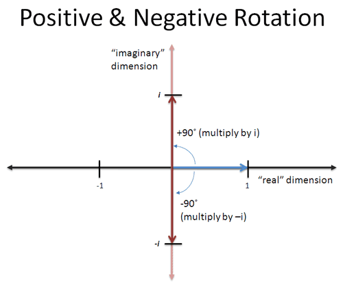
Complex numbers are just rotations.
Let's start with a set $S_1 = \{ 1 \}$. What set can collapse into this set?
Easy, $S_2 = \{-1, 1\}$. What set collapses to $S_2$?
Easy, $S_3 = \{i, -i, 1, -1\}$. What set collapses to $S_3$?
Not so easy (until you read Kalid's post!), but it's $S_4 = \{\frac{\sqrt{2}}{2}(1 + i), -\frac{\sqrt{2}}{2}(i + i), \frac{\sqrt{2}}{2}(i - 1), -\frac{\sqrt{2}}{2}(i + 1), i, -i, 1, -1\}$.
We can keep going. In essence, we can always find a set that collapses like this, for any even n, however big! Take a minute, that is like wow!
Formally, a set containing $n$ points that collapse as shown above, are called the nth roots of unity. If we square these $n$ points, n times, we get 1 (The basecase of our recursion)!
Running time of our Divide and Conquer Algorithm
Ok, let's just step back and see how well our divide and conquer algorithm would perform.
- We take our polynomial $A(x)$, to be evaluated on a set $X$ with $|X| = n$, and reduce it to two smaller problems.
- $A_{even}(x)$ and $A_{odd}(x)$, both evaluated on set $Y = \{x^2 | x \in X\}$ with $|Y| = n/2$.
We can write a recurrence relation for the above algorithm as:
$T(n) = 2T(\frac{n}{2}) + O(n)$
where $T(n)$ is the running time of our algorithm on an input of size $n$. Solving this, we get a runtime bound of O(n lgn)
Cool! We can now Add, Evaluate and Multiply polynomials in $O(n lg n)$ time!
*This elegant divide and conquer algorithm, is the FFT algorithm!
I hope this helps you understand what the FFT is all about. In a future post, we will discuss how its implemented, where the $e^{i\theta}$ and fourier related terms come in.