Understanding Entropy, Cross-Entropy, and KL Divergence
Table of Contents
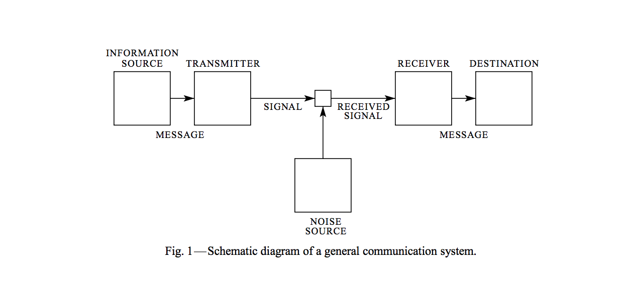
Back in 1948, Claude Shannon published his master's thesis, A Mathematical Theory of Communication, essentially inventing information theory in the process. He introduced a simple diagram showing how communication systems work:
Then he defined Entropy — a concept that became the foundation for everything we do with information today.
What is Entropy Anyway?
Information entropy gets explained in many ways, but here's my favorite: "How much randomness is floating around in your data?" It's similar to Boltzmann's Entropy from physics, if you're familiar with that.
The formula looks like this:
\[ H = -K \sum_{i = 1}^{n} p_i \log{p_i} \]
where \(p_i\) is the probability of event i happening. (The constant K just lets you choose your units — bits, nats, whatever works for you.)
A Weather Example
Let me show you what this actually means with some weather data:
import numpy as np
H = lambda xs: -numpy.sum(map(lambda x: x * numpy.log2(x) if x != 0 else 0, xs))
return list(map(H, [[0.25, 0.25, 0.25, 0.25], [0.5, 0.2, 0.2, 0.1],
                     [0.8, 0.1, 0.05, 0.05], [1, 0, 0, 0]]))
| Sunny | Rainy | Snowy | Foggy | Entropy |
|---|---|---|---|---|
| 0.25 | 0.25 | 0.25 | 0.25 | 2.0 |
| 0.5 | 0.2 | 0.2 | 0.1 | 1.76 |
| 0.8 | 0.1 | 0.05 | 0.05 | 1.02 |
| 1 | 0 | 0 | 0 | 0 |
See the pattern? The more uncertain things are, the higher the entropy. When you know something will happen for sure (like that last row with 100% sunny weather), entropy drops to zero. Makes sense, right?
Why Should You Care?
Notice I used base 2 for the logarithm? When you do that, Shannon called the units bits (J. W. Tukey apparently came up with that name). So you can think of entropy as answering this question:
On average, how many bits do I need to send this information?
This insight proved incredibly useful for building efficient communication systems. The basic principle: if something happens frequently, use fewer bits to represent it. If it's rare, you can afford to use more bits.
But knowing the theoretical minimum is just the starting point. How do you know if your actual system is any good? That's where cross-entropy comes in.
Cross-Entropy: Measuring Real-World Performance
\[ H(p, q) = -K \sum_{i = 1}^{n} p_i \log{q_i} \]
Here, \(q_i\) is what your system thinks the probability is, while \(p_i\) is the actual probability in the real world.
I think of cross-entropy as answering: "How many bits is your system actually using?" (as opposed to the theoretical minimum).
The elegant part? If your system is perfect and \(q_i = p_i\) for all events, then cross-entropy equals regular entropy. Your system is as efficient as theoretically possible.
KL Divergence: The Efficiency Gap
The difference between cross-entropy and entropy is called Relative Entropy or KL Divergence. It tells you exactly how far you are from perfect efficiency:
\[ D_{KL}(p || q) = H(p, q) - H(p) \]
Higher KL divergence means you're wasting more bits — your system isn't as efficient as it could be.
Why Machine Learning Loves Cross-Entropy
Cross-entropy shows up everywhere in machine learning as a loss function, especially for classification problems. Here's a detailed example if you want to explore further.
The intuition is straightforward:
- Model is confident and correct: Cross-entropy is low ✓
- Model is confident but wrong: Cross-entropy shoots up ✗
- Model is uncertain about everything: Cross-entropy is somewhere in between ~
It's the perfect way to penalize both overconfident wrong predictions and general uncertainty — exactly what you want when training a classifier.